
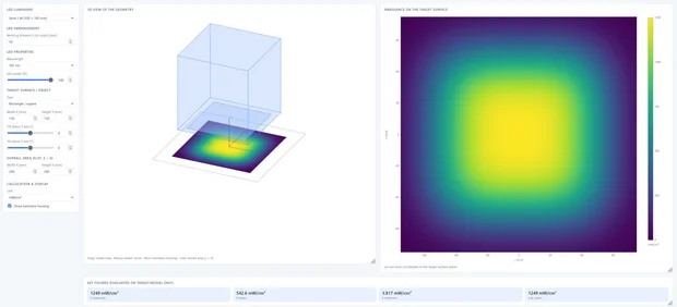
The UV LED irradiance calculator by Opsytec Dr. Gröbel simulates the irradiance (mW/cm²) of UV LED luminaires directly in your browser — free of charge, no installation required. Choose a UV LED flood lamp or a Series L luminaire, set the wavelength (265–450 nm), the working distance and the target area, and instantly get the irradiance distribution as a heatmap, a 3D view and cross-section profiles — optionally on your own parts imported as STEP/STL models.
The simulation uses the measured emission characteristics of real UV LEDs and reports key figures such as maximum, average and minimum irradiance for designing UV curing, UV disinfection, weathering and fluorescence applications. Results can be exported as CSV files and as a PDF simulation report. The calculated values are indicative data for product selection; binding irradiance levels should be verified by measurement, e.g. with an Opsytec radiometer.
Model: LED sources (5 sub-sources per LED) with the measured OPSY1 emission characteristic (θ½ = ±32°) or optionally the Lambertian model I(θ) = I₀·cosᵐθ. Irradiance E = Σ I(θ_LED)·cos(θ_incidence)/r². The pivot/model origin lies at working distance h below the LED plane; the overall area is flat at z = 0. For CAD models, E is computed per outer face (triangle); back faces receive E = 0. Reflections, Fresnel losses and self-shadowing are not considered.
Fundamentals of the UV LED simulation
Select a predefined UV LED luminaire (SFL flood lamp or Series L) and the desired wavelength — the matching radiant flux per LED is stored for every wavelength. Set the working distance between the LED plane and the target, and define the target as a rectangle, a circle or your own CAD model (STEP/STL, processed entirely locally in your browser). The app computes the irradiance distribution and displays it as an interactive 3D view, a heatmap and cross-section profiles through the centre. Key figures such as maximum, average and minimum irradiance and the value at the centre are shown directly; all results can be exported as CSV files or as a PDF simulation report.
Each UV LED is modelled as a compact source of five sub-sources across the die. The irradiance at a point on the target is the incoherent sum of all LED contributions: E = Σ I(θ) · cos(θinc) / r². By default the emission characteristic I(θ) is the OPSY LED model (half angle ±32°), validated against measurement data and Monte-Carlo ray tracing; alternatively the classic Lambertian model I(θ) = I₀·cosᵐθ with adjustable half angle is available. Both models are energy-normalised: the flux integrated over the hemisphere equals exactly the configured flux per LED.
- Working distance: in the far field the irradiance falls with 1/r²; at the same time the individual LED contributions overlap more with increasing distance, making the distribution more uniform. Short distances give high peak values with a visible LED pattern.
- LED count and pitch: more LEDs and a smaller pitch increase irradiance and uniformity; towards the edge of the array the irradiance inherently drops off.
- Wavelength: the available radiant flux per LED depends on the wavelength — UVC LEDs (265–280 nm) deliver considerably less power than UVA LEDs (365–450 nm).
- Target tilt: a surface tilted about the X or Y axis receives less irradiance according to the cosine of the angle of incidence.
The simulation assumes direct irradiation in an unobstructed half-space: reflections from surrounding surfaces, Fresnel losses at the part surface and self-shadowing inside concave geometries are not taken into account; for CAD models, faces turned away from the LEDs receive zero. The results are therefore indicative data for product selection and process design — without warranty. Binding irradiance and dose values should be determined by measurement with a calibrated UV radiometer from Opsytec Dr. Gröbel.
All simulated luminaires are series products of Opsytec Dr. Gröbel GmbH: the SFL series UV LED flood lamps irradiate large areas homogeneously — for UV curing, fluorescence excitation and disinfection — while the compact Series L UV LED luminaires generate high irradiance on small areas. Both series are available with wavelengths from 265 nm to 450 nm. We are happy to help you select and design the right UV irradiation unit for your application.
Frequently asked questions
The simulation uses measured LED emission characteristics and is validated against Monte-Carlo ray tracing. It provides indicative data for product selection; reflections and Fresnel losses are not included. Binding values should be determined by measurement with a calibrated UV radiometer.
Short distances maximise irradiance but show the LED pattern as non-uniformity; larger distances smooth the distribution at lower irradiance. Compare several distances in the simulation using the cross-section profiles and the "E average" key figure to find the best compromise for your application.
Yes — load a STEP or STL model of your part. The irradiance is computed per outer face; faces turned away from the LEDs receive zero. The file is processed entirely locally in your browser and is never uploaded.
The simulation covers 265, 275, 280, 365, 385, 395, 405 and 450 nm — from UVC for disinfection to UVA/blue for curing and fluorescence. The typical radiant flux per LED is stored for every wavelength and used automatically in the calculation.
Author: Dr. Mark Paravia
Dr.-Ing. Mark Paravia is the managing director of Opsytec Dr. Gröbel GmbH in Ettlingen and heads the accredited calibration laboratory. Following his research on pulsed xenon excimer discharges at the Institute of Lighting Technology at KIT, his current focus is on optical radiation measurement technology. He is a recognized UV expert, vice-chair of the DIN Standards Committee FNL 7 “Optical Radiation,” and a member of the DVGW Project Group on UV Disinfection.